At work, I am responsible for collecting PLC/HMI data logs from systems, organizing and transforming the data so relative system performance can be acquired.
In the infancy of my “data science” journey, I used Microsoft Excel and its integrated Power Query program to fulfill my data analysis needs. This method had a very shallow learning curve and was for the most part graphical. I ended up using this method for the first few projects. It wasn’t until more complex projects with larger data sets that I hit the limitations of Excel’s row limit as well as the computational bottleneck of Power Query.
For my most recent project I used Power Query in Excel up until around 700,000 rows. With Excel’s 1,048,576 row limit imminently approaching, I began searching for solution that could handle the vast amounts of data that would accumulate as I was only about 3 months into a multi year project.
I then stumbled upon Microsoft Power Bi, which is usually used for business intelligence and generally revenue based data and decided to give it a shot.

Power Bi was an impressively powerful and robust tool for visualizing massive quantities of data and has various data source integrations. However its core data transformation tool consisted of Power Query, which was just too limited in functionality and vastly inefficient when large quantities of data are involved. My 700k row data file took roughly 20-30 minutes to finish transforming, this would not be acceptable when more data started to accumulate.
I looked around and ended up finding some references of people using Python and Pandas for big data. There was a steeper learning curve then Power Query since there was no GUI available and all the transformations needed to be coded, but the end result was a lightning fast and robust data cleaning and transformation tool that could handle recursive calculations with ease (something Power Query struggled with and was necessary in my application). However pandas did not have all the functionality I needed and I had to install numpy and glob.
Below is the full code to my cleaning function.
| import pandas as pd | |
| import glob | |
| import datetime | |
| import sys | |
| import os | |
| import os.path | |
| from os import listdir | |
| from os.path import isfile, join | |
| import glob | |
| import re | |
| import numpy as np | |
| print("Looking for Old Transformation File") | |
| if os.path.exists('Cleaned Data.csv'): | |
| print("Old File Found") | |
| print("Removing Old Transformation File") | |
| os.remove("Cleaned Data.csv") | |
| else: | |
| print("Transformation File Does Not Exist") | |
| pd.set_option('display.max_rows',1000) | |
| pd.set_option('display.max_columns', 500) | |
| pd.set_option('display.width', 1000) | |
| my_path = os.path.abspath('') | |
| Analog = os.path.join(my_path, "Raw","Full Analog","*.csv").replace("\\","/") | |
| Backwash =os.path.join(my_path,"Raw","Full Backwash","*.csv").replace("\\","/") | |
| OM = os.path.join(my_path,"Raw","Full Operation Mode","*.csv").replace("\\","/") | |
| print("Importing and Combining All Files in Folder...") | |
| print(Analog) | |
| print(Backwash) | |
| print(OM) | |
| all_analog = glob.glob(Analog) | |
| all_backwash=glob.glob(Backwash) | |
| all_om=glob.glob(OM) | |
| li1 = [] | |
| li2 = [] | |
| li3 = [] | |
| for filename in all_analog: | |
| df1 = pd.read_csv(filename, index_col=False,low_memory=False) | |
| li1.append(df1) | |
| df1 = pd.concat(li1, axis=0, ignore_index=True) | |
| for filename in all_backwash: | |
| df2 = pd.read_csv(filename, index_col=False,low_memory=False) | |
| li2.append(df2) | |
| df2 = pd.concat(li2, axis=0, ignore_index=True) | |
| for filename in all_om: | |
| df3 = pd.read_csv(filename, index_col=False,low_memory=False) | |
| li3.append(df3) | |
| df3 = pd.concat(li3, axis=0, ignore_index=True) | |
| df1['Time'] = pd.to_datetime(df1['Time'].astype(str), format= "%Y %m %d %H:%M:%S") | |
| df2['Time'] = pd.to_datetime(df2['Time'].astype(str), format= "%Y %m %d %H:%M:%S") | |
| df3['Time'] = pd.to_datetime(df3['Time'].astype(str), format= "%Y %m %d %H:%M:%S") | |
| df1.set_index('Time') | |
| df2.set_index('Time') | |
| df3.set_index('Time') | |
| df_outer = pd.merge(df1,df2, on='Time', how='outer',sort=True) | |
| df_outer = pd.merge(df_outer,df3, on='Time',how='outer',sort=True) | |
| df_outer=df_outer.fillna(method='ffill') | |
| df4=df_outer | |
| print("Cleaning Analog, Backwash, and Operation Mode Data") | |
| df4['[B] Wet Weather Step Description'] = np.where((df4['BBF2.WET_WEATHER.STEP']==3.0), "Filtering", | |
| np.where((df4['BBF2.WET_WEATHER.STEP']==5.0), "Backwashing", | |
| np.where((df4['BBF2.WET_WEATHER.STEP']==2.0),"Start of Filtering", | |
| np.where((df4['BBF2.WET_WEATHER.STEP']==6.0), "End of Backwash", | |
| np.where((df4['BBF2.WET_WEATHER.STEP']==4.0),"End of Filtering", | |
| np.where((df4['BBF2.WET_WEATHER.STEP']==0),"Idle",None)))))) | |
| df4['[F] Primary Step Description'] = np.where((df4['BBF1.PRIMARY.STEP']==3.0), "Filtering", | |
| np.where((df4['BBF1.PRIMARY.STEP']==5.0), "Backwashing", | |
| np.where((df4['BBF1.PRIMARY.STEP']==2.0),"Start of Filtering", | |
| np.where((df4['BBF1.PRIMARY.STEP']==6.0), "End of Backwash", | |
| np.where((df4['BBF1.PRIMARY.STEP']==4.0),"End of Filtering", | |
| np.where((df4['BBF1.PRIMARY.STEP']==0),"Idle",None)))))) | |
| df4['[F] Wet Weather Step Description'] = np.where((df4['BBF1.WET_WEATHER.STEP']==3.0), "Filtering", | |
| np.where((df4['BBF1.WET_WEATHER.STEP']==5.0), "Backwashing", | |
| np.where((df4['BBF1.WET_WEATHER.STEP']==2.0),"Start of Filtering", | |
| np.where((df4['BBF1.WET_WEATHER.STEP']==6.0), "End of Backwash", | |
| np.where((df4['BBF1.WET_WEATHER.STEP']==4.0),"End of Filtering", | |
| np.where((df4['BBF1.WET_WEATHER.STEP']==0),"Idle",None)))))) | |
| df4['[B] Primary Step Description'] = np.where((df4['BBF2.PRIMARY.STEP']==3.0), "Filtering", | |
| np.where((df4['BBF2.PRIMARY.STEP']==5.0), "Backwashing", | |
| np.where((df4['BBF2.PRIMARY.STEP']==2.0),"Start of Filtering", | |
| np.where((df4['BBF2.PRIMARY.STEP']==6.0), "End of Backwash", | |
| np.where((df4['BBF2.PRIMARY.STEP']==4.0),"End of Filtering", | |
| np.where((df4['BBF2.PRIMARY.STEP']==0),"Idle",None)))))) | |
| df4['[B] Backwash Step Description'] = np.where((df4['BBF2.BACKWASH.STEP']==0), "Not in BW", | |
| np.where((df4['BBF2.BACKWASH.STEP']==2.0),"Step 1: Idle", | |
| np.where((df4['BBF2.BACKWASH.STEP']==3.0), "Step 2: Drain", | |
| np.where((df4['BBF2.BACKWASH.STEP']==4.0),"Step 3: Idle", | |
| np.where((df4['BBF2.BACKWASH.STEP']==5.0),"Step 4: Air", | |
| np.where((df4['BBF2.BACKWASH.STEP']==6.0),"Step 5: Idle", | |
| np.where((df4['BBF2.BACKWASH.STEP']==7.0),"Step 6: Drain", | |
| np.where((df4['BBF2.BACKWASH.STEP']==8.0),"Step 7: Idle", | |
| np.where((df4['BBF2.BACKWASH.STEP']==9.0),"Step 8: Drain", | |
| np.where((df4['BBF2.BACKWASH.STEP']==10.0),"Step: 9 Idle", | |
| np.where((df4['BBF2.BACKWASH.STEP']==11.0),"Step 10: Drain", | |
| np.where((df4['BBF2.BACKWASH.STEP']==12.0),"Step 11: Idle",None)))))))))))) | |
| df4['[F] Backwash Step Description'] = np.where((df4['BBF1.BACKWASH.STEP']==0), "Not in BW", | |
| np.where((df4['BBF1.BACKWASH.STEP']==2.0),"Step 1: Idle", | |
| np.where((df4['BBF1.BACKWASH.STEP']==3.0), "Step 2: Drain", | |
| np.where((df4['BBF1.BACKWASH.STEP']==4.0),"Step 3: Idle", | |
| np.where((df4['BBF1.BACKWASH.STEP']==5.0),"Step 4: Air", | |
| np.where((df4['BBF1.BACKWASH.STEP']==6.0),"Step 5: Idle", | |
| np.where((df4['BBF1.BACKWASH.STEP']==7.0),"Step 6: Drain", | |
| np.where((df4['BBF1.BACKWASH.STEP']==8.0),"Step 7: Idle", | |
| np.where((df4['BBF1.BACKWASH.STEP']==9.0),"Step 8: Drain", | |
| np.where((df4['BBF1.BACKWASH.STEP']==10.0),"Step: 9 Idle", | |
| np.where((df4['BBF1.BACKWASH.STEP']==11.0),"Step 10: Drain", | |
| np.where((df4['BBF1.BACKWASH.STEP']==12.0),"Step 11: Idle",None)))))))))))) | |
| df4['[B] Recirculation Step Description'] = np.where((df4['BBF2.RECIRC.STEP']==2.0),"Recirculating","Idle") | |
| df4['[F] Recirculation Step Description'] = np.where((df4['BBF1.RECIRC.STEP']==2.0),"Recirculating","Idle") | |
| df4 = df4.rename(columns={'SENSORS.INFLUENT.SST': 'newName1'}) | |
| df4.drop(([df4.columns[1],df4.columns[15],df4.columns[16],df4.columns[30]]),axis=1,inplace=True) | |
| df4 = df4.rename(columns={df4.columns[0]: 'DateTime', | |
| df4.columns[1] : "[LF] Influent ORP (mV)", | |
| df4.columns[2] : "[F] Reactor DO (ppm)", | |
| df4.columns[3] : "[F] Reactor pH", | |
| df4.columns[4] : "[F] Reactor Temp (F)", | |
| df4.columns[5] : "[F] Effulent TSS (ppm)", | |
| df4.columns[6] : "[F] Reactor Pressure (psi)", | |
| df4.columns[7] : "[F] Influent Flow (gpm)", | |
| df4.columns[8] : "[B] Reactor DO (ppm)", | |
| df4.columns[9] : "[B] Reactor pH", | |
| df4.columns[10] : "[B] Reactor Temp (F)", | |
| df4.columns[11] : "[B] Effulent TSS (ppm)", | |
| df4.columns[12] : "[B] Reactor Pressure (psi)", | |
| df4.columns[13] : "[B] Influent Flow (gpm)", | |
| df4.columns[14] : "[Coag] Stock Solution Conc. (ppm)", | |
| df4.columns[15] : "[Coag] Influent Final Conc. SP (ppm)", | |
| df4.columns[16] : "[Coag] ", | |
| df4.columns[17] : "[Poly] Stock Solution Conc. (ppm)", | |
| df4.columns[18] : "[Poly] Influent Final Conc. SP (ppm)", | |
| df4.columns[19] : "[Poly] ", | |
| df4.columns[20] : "[HF] Pump Hz", | |
| df4.columns[21] : "[LF] Pump Hz", | |
| df4.columns[22] : "[Coag] Pump Flowrate (mL/min)", | |
| df4.columns[23] : "[Poly] Pump Flowrate (mL/min)", | |
| df4.columns[24] : "[HF] Influent TSS (ppm)", | |
| df4.columns[25] : "[LF] Influent TSS (ppm)", | |
| df4.columns[26] : "[LF] Influent Temperature (F)", | |
| df4.columns[27] : "[B] Effulent ORP (mV)", | |
| df4.columns[28] : "[F] Reactor Linear Velocity (m/hr)", | |
| df4.columns[29] : "[B] Reactor EBCT (min)", | |
| df4.columns[30] : "[B+F] Backwash Flowrate (gpm)", | |
| df4.columns[31] : "[F] Primary Step Number", | |
| df4.columns[32] : "[F] Backwash Step Number", | |
| df4.columns[33] : "[F] Wet Weather Step Number", | |
| df4.columns[34] : "[F] Recirculation Step Number", | |
| df4.columns[35] : "[B] Backwash Step Number", | |
| df4.columns[36] : "[B] Primary Step Number", | |
| df4.columns[37] : "[B] Wet Weather Step Number", | |
| df4.columns[38] : "[B] Recirculation Step Number"}) | |
| df4.drop(([df4.columns[16],df4.columns[19]]),axis=1,inplace=True) | |
| df4['Time Delta (min)'] = df4['DateTime'].shift(-1)-df4['DateTime'] | |
| df4['Time Delta (min)'] = df4['Time Delta (min)'].dt.total_seconds()/60 | |
| avgfin= (df4['[F] Influent Flow (gpm)']+df4['[F] Influent Flow (gpm)'].shift(-1))/2 | |
| avgbin= (df4['[B] Influent Flow (gpm)']+df4['[B] Influent Flow (gpm)'].shift(-1))/2 | |
| avgbw = (df4['[B+F] Backwash Flowrate (gpm)']+df4['[B+F] Backwash Flowrate (gpm)'].shift(-1))/2 | |
| df4['[F] Reactor Pressure during Filtration (psi)'] = np.where((df4[df4.columns[38]]=="Filtering"),df4[df4.columns[6]], None) | |
| df4['[F] Reactor Linear Velocity during Filtration (m/hr)']=np.where((df4[df4.columns[38]]=="Filtering"),df4[df4.columns[26]],None) | |
| df4['[F] Influent TSS during Filtration (ppm)'] = np.where((df4[df4.columns[38]]=="Filtering")&(df4[df4.columns[22]]<2000)&(df4[df4.columns[22]]>0),df4[df4.columns[22]], np.where((df4[df4.columns[31]]=="Filtering")&(df4[df4.columns[23]]<2000)&(df4[df4.columns[23]]>0),df4[df4.columns[23]],None)) | |
| df4['[F] Effulent TSS during Filtration (ppm)'] = np.where((df4[df4.columns[38]]=="Filtering")&(df4[df4.columns[5]]<2000)&(df4[df4.columns[5]]>0),df4[df4.columns[5]],None) | |
| df4['[F] TSS Removal during Filtration (%)'] = np.where((df4[df4.columns[48]]>0)&(df4[df4.columns[49]]>0),1-(df4[df4.columns[49]]/df4[df4.columns[48]]),None) | |
| df4['[F] Filtration Volume (gal)'] = np.where((df4[df4.columns[38]]=="Filtering"),avgfin*df4['Time Delta (min)'], None) | |
| df4['[F] Backwash Volume (gal)'] = np.where((df4[df4.columns[42]].str.contains('Drain', case=True,regex=True)),avgbw*df4['Time Delta (min)'],None) | |
| df4['[F] Idle Duration (min)'] = np.where((df4[df4.columns[42]].str.contains('Idle', case=True,regex=True)),df4['Time Delta (min)'],None) | |
| df4['[F] Drain Duration (min)'] = np.where((df4[df4.columns[42]].str.contains('Drain', case=True,regex=True)),df4['Time Delta (min)'],None) | |
| df4['[F] Air Duration (min)'] = np.where((df4[df4.columns[42]].str.contains('Air', case=True,regex=True)),df4['Time Delta (min)'],None) | |
| df4['[F] Backwash Duration (min)'] = np.where((df4[df4.columns[42]]!='Not in BW')&(df4[df4.columns[42]].notnull()),df4['Time Delta (min)'],None) | |
| df4['[B] Influent ORP during Filtration (mV)'] = np.where((df4[df4.columns[37]]=="Filtering"),df4[df4.columns[1]], None) | |
| df4['[B] Effulent ORP during Filtration (mV)'] = np.where((df4[df4.columns[37]]=="Filtering"),df4[df4.columns[25]], None) | |
| df4['[B] Reactor Pressure during Filtration (psi)'] = np.where((df4[df4.columns[37]]=="Filtering"),df4[df4.columns[12]], None) | |
| df4['[B] Reactor Linear Velocity during Filtration (m/hr)']=np.where((df4[df4.columns[37]]=="Filtering"),0.1945525292*df4[df4.columns[13]],None) | |
| df4['[B] Influent TSS during Filtration (ppm)'] = np.where((df4[df4.columns[37]]=="Filtering")&(df4[df4.columns[23]]<2000)&(df4[df4.columns[23]]>0),df4[df4.columns[23]], np.where((df4[df4.columns[34]]=="Filtering")&(df4[df4.columns[22]]<2000)&(df4[df4.columns[22]]>0),df4[df4.columns[22]],None)) | |
| df4['[B] Effulent TSS during Filtration (ppm)'] = np.where((df4[df4.columns[37]]=="Filtering")&(df4[df4.columns[11]]<2000)&(df4[df4.columns[11]]>0),df4[df4.columns[11]],None) | |
| df4['[B] TSS Removal during Filtration (%)'] = np.where((df4[df4.columns[62]]>0)&(df4[df4.columns[61]]>0),1-(df4[df4.columns[62]]/df4[df4.columns[61]]),None) | |
| df4['[B] Filtration Volume (gal)'] = np.where((df4[df4.columns[37]]=="Filtering"),avgbin*df4['Time Delta (min)'], None) | |
| df4['[B] Filtration Duration (gal)'] = np.where((df4[df4.columns[37]]=="Filtering"),df4['Time Delta (min)'], None) | |
| df4['[B] Backwash Volume (gal)'] = np.where((df4[df4.columns[41]].str.contains('Drain', case=True,regex=True)),avgbw*df4['Time Delta (min)'],None) | |
| df4['[B] Idle Duration (min)'] = np.where((df4[df4.columns[41]].str.contains('Idle', case=True,regex=True)),df4['Time Delta (min)'],None) | |
| df4['[B] Drain Duration (min)'] = np.where((df4[df4.columns[41]].str.contains('Drain', case=True,regex=True)),df4['Time Delta (min)'],None) | |
| df4['[B] Air Duration (min)'] = np.where((df4[df4.columns[41]].str.contains('Air', case=True,regex=True)),df4['Time Delta (min)'],None) | |
| df4['[B] Backwash Duration (min)'] = np.where((df4[df4.columns[41]]!='Not in BW')&(df4[df4.columns[41]].notnull()),df4['Time Delta (min)'],None) | |
| df4['[B] Empty Bed Contact Time (min)']=np.where((df4[df4.columns[37]]=="Filtering"),df4['[B] Reactor EBCT (min)'],None) | |
| df4['[F] Empty Bed Contact Time (min)']=np.where((df4[df4.columns[38]]=="Filtering"),616.84364/df4['[F] Influent Flow (gpm)'],None) | |
| df4['[F] Filtration Duration (min)'] = np.where((df4[df4.columns[38]]=="Filtering"),df4['Time Delta (min)'], None) | |
| df4['Tandum Backwash'] = np.where((df4[df4.columns[37]]=="Backwashing") & (df4[df4.columns[38]]=='Backwashing'),True,None) | |
| df4['[F] New Cycle'] = np.where((df4[df4.columns[38]]=='Start of Filtering')|(df4[df4.columns[39]]=='Start of Filtering'),True,None) | |
| df4['[B] New Cycle'] = np.where((df4[df4.columns[37]]=='Start of Filtering')|(df4[df4.columns[40]]=='Start of Filtering'),True,None) | |
| df4['[F] Backwash Count'] = np.where(((df4[df4.columns[38]]=='Backwashing')&(df4[df4.columns[38]].shift(-1)!='Backwashing'))|((df4[df4.columns[39]]=='Backwashing')&(df4[df4.columns[39]].shift(-1)!='Backwashing')),True,None) | |
| df4['[B] Backwash Count'] = np.where(((df4[df4.columns[37]]=='Backwashing')&(df4[df4.columns[37]].shift(-1)!='Backwashing'))|((df4[df4.columns[40]]=='Backwashing')&(df4[df4.columns[40]].shift(-1)!='Backwashing')),True,None) | |
| Date, Time = zip(*[(d.date(), d.time()) for d in df4['DateTime']]) | |
| df4 = df4.assign(Date=Date, Time=Time) | |
| df4 = df4.rename(columns={df4.columns[0]: 'Date/Time'}) | |
| df5 = pd.read_csv("Test Number Dates.csv", index_col=False,low_memory=False) | |
| df5['Date/Time'] = pd.to_datetime(df5['Date/Time'].astype(str), format= "%m/%d/%Y %H:%M") | |
| df4.set_index('Date/Time') | |
| df5.set_index('Date/Time') | |
| df4 = pd.merge_asof(df4,df5, on='Date/Time', direction='backward') | |
| df4['Test Number']=df4['Test Number'].fillna(method='ffill') | |
| print("Saving Data to CSV") | |
| df4.to_csv("Cleaned Data.csv") | |
| print(str(len(df4.index))+" Rows Exported") |
First in lines 27 through 30, I used os.path the retrieve my absolute path in order to allow the python module to be run from any location so long as the folder structure that the raw CSV data is located in is correct. I had some issues with “\” registering with python so I had to replace it with “/” (when referencing the character “\” you must put another forward slash informant “\\”). I then assigned variables to the three paths where my CSV files where located giving the ending path a “*” wild card variable, allowing all CSV files in the path to be referenced.
Lines 37 to 39, assigned variables and globed those CSV files with glob.glob
Lines 41 to 62, I appended each categories CSV’s into a single array and saved them into 3 respective data frames in pandas.
Lines 64 to 70, converted the non time stamp string format into a pandas timestamp and set each data frames index to the converted time stamp.
Lines 72 to 75, merged all three data frames together using a outer merge and filled down so that no cells had missing data. This method was done since the data set for Analog logged at 1 minute intervals consistently, Backwash every 1 second during a value change, and Operational Mode when ever a value was changed. This caused a several unique index values that were independent to each data set.
Lines 70 to 134, created additional columns that describe what step the unit was in based on a integer value.
Lines 136 to 183, removed and renamed all the columns. You can either reference the columns by their numeric index value or their name.
Lines 184 and 185, created a column that represented the recursive difference between the current and next time stamp and converted the value to minutes so that duration and volume based calculations could take place.
Lines 187 to 235, created conditional calculation columns that have values during certain scenarios for the ease of data use in Power Bi.
Lines 237 to 243, were added at a later revision. These lines of code imported a CSV file which had date times that I had assigned “Test Numbers” to in order to provide an index-able value to correlate to a testing schedule that I would import into Power Bi. I began by importing the CSV to a data frame and then converting the time stamp to a pandas date stamp and then setting that to the index. I then used pd.mergeasof to merge the two data frames, with the augment backwards, and filled down so that each row had a index-able “Test Number”.
Lines 245 to 247, printed to console that the module was saving the resulting data set into a CSV format, explorted via the df.to_csv command, and printed the number of rows exported.
With that the Python/Pandas portion of the data transformation portion was finished.
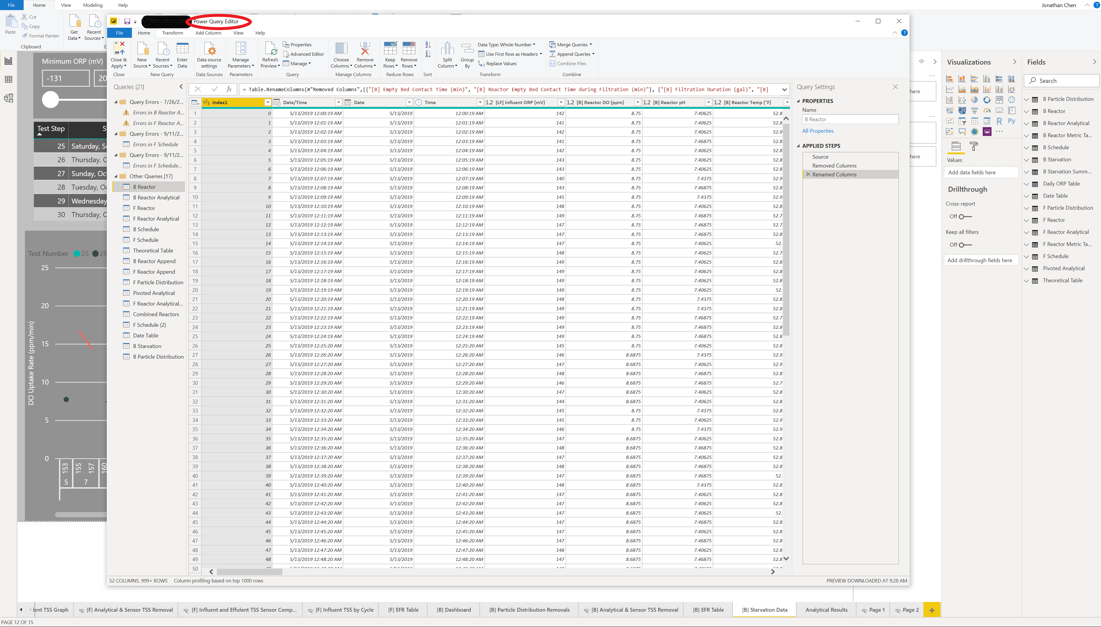
The next step was importing the “Cleaned CSV” into Power Bi and begin the final steps of data cleaning in Power Query.
The “Cleaned CSV” actually consisted of two separate units that were logged into one file, in Power Query I made 2 new referenced queries that separated these two data files, maintaining their time stamps which I had to separate into: Date/Time, Date, and Time. This was done due to the limitation of Power Bi to handle date hierarchies that included times and to prevent conflict with relating data sets that only consisted of date stamps.
From there I imported a number of associated files such as: Testing Schedule, Analytical Laboratory Data, and a Date Table. This data was then cleaned, separated and formatted for each of the two units. I also created a pivoted version of the analytical data so that a dynamic series could be used in one of my visuals.

Doing this allowed for a specific attribute to be selected and displayed on a graph rather then manually dragging and dropped the attribute from the data set every time a new attribute needed to be plotted.
The next step of the data cleaning and transformation took place in the DAX environment of Power Bi after the data import from Power Query was done. I needed to number “cycles” that our unit had been through based on certain conditions. i.e. a cycle for gas usage for your car would be driving your car X amount of miles then filling up your gas tank. You can then use the number of miles you drive and divide it by the number of gallons you filled up to determine gas mileage, given that you fill up your tank to full every time. In order to achieve this I had already created a column that displayed the state the unit was in, in its next row. This all I needed to do is create a logical function that compared the current row to the column that had the row shifted by +1 to logically determine if it was a “new cycle”. But the hardest part was numbering each of these cycles in an incremental manner and applying it to every row in that “cycle”. After several hours of googling I found the perfect function that would get the job done. It is the magical RANKX DAX function paired with a FILTER function.
I then used this to create a separate table that would summarize all the data for each “cycle”, with the SUMMERIZECOLUMNS DAX function. This allowed me to calculate metrics by each cycle rather then by date or time.
The final step of the data transformation and cleaning was defining relationship between the 16 individual data sets I had using Power Bi’s relationship tool. This part was quite frustrating because of many discontinuity errors but I found a solution which involved the “Test Number” I added in to the Pandas transform and a Date Table.
Now I have over 2 million rows of primary operation data that is directly referable to test plans, analytical data, metrics, and any other data sets I decided to add in the future.