Background
SHA-3 is short for Secure Hash Algorithm 3 This means that SHA-3 is a hash function and meets certain attack resistance criteria, if you don’t know what those are you can read my introduction post on hashing functions. I will go into depth about hashing function attacks and what makes a hashing function secure as well as how previous functions were defeated in a later post.
This post covers step by step how SHA-3 takes in data and creates a hashed output. SHA-3 is most popularly used in Ethereum(ETH) via its Keccak-256 flavor.
I wrote this post mainly because it was pretty hard for me to break down SHA-3 coming from a Chemical Engineering background and there were really no posts out there that tried to explain it to someone without a strong Computer Science/Mathematics background.
Sponge Construction
The SHA-3 algorithm is unique to other SHA functions due to the fact it uses an approach called sponge construction. After trying to make sense of a few diagrams, I decided to create a version that made more sense to me.
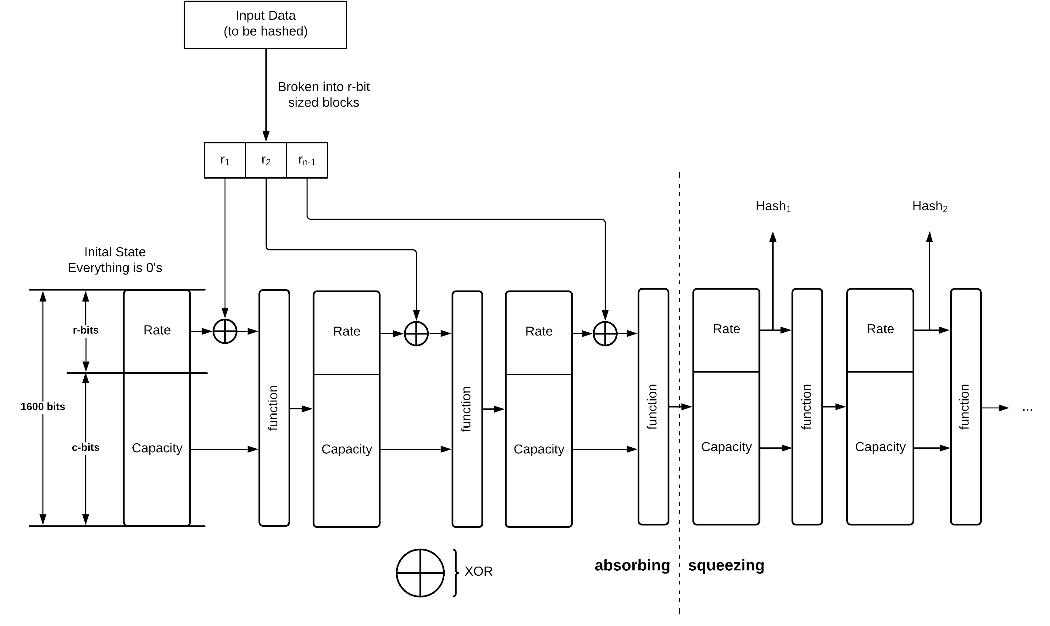
SHA-3’s sponge construction works by:
- Breaking the input data to be hashed into r-bit sized chunks, in SHA-3’s case the rate+capacity bits sum up to 1600 bits.
- The first input rate and capacity are all zeros and are XORed with the first rate block r1
- The combined rate and capacity block is put through a function, usually of multiple rounds.
- The first r-bits of the function are rate and the remaining c-bits capacity.
- The above r-bits are XORed with r2 and fed into another function
- This is done until there are no left over data blocks.
- On the last data block, the hash is taken from r-bits output of the function.
- If more bits are needed the above rate and capacity are fed through the function without inputing any additional data.
Padding
Since data is rarely perfectly divided into an equal number of blocks perfectly, SHA-3 must pad the input data to be perfectly divisible by r-bits. This padding is done by adding a 1 bit, then filling in with zero or more 0’s and then ending with a 1 bit. The two cases for input padding are described below.

In the case of the inputs being perfectly divisible into r-bits we use case 2 as shown above. This is done to make sure that a message with length divisible by r-bits that ends in something that that looks like padding does not produce the same hash as the message with those bits removed.
The Keccak Function
The Keccak function is the heart of SHA-3, this function is the function block in the above diagram, it uses XOR, AND and NOT operations which translate into easy implementation in both software and hardware scenarios.
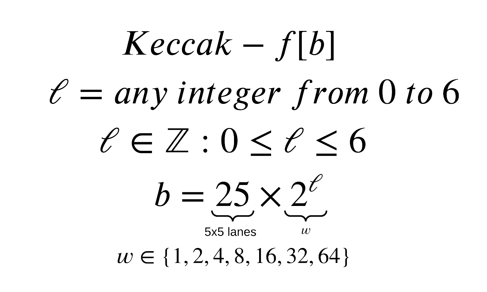
∈ – Element of, means that it is a part of the next set of numbers
ℤ – Represents the family of Integers
b – number of bits the function takes
ℓ – is any integer from 0 to 6, the main SHA-3 implementation uses a ℓ value of 6.
Explaining the mathematical notation of line 3 in plain english.
ℓ is a member of the family of integers, it needs to be a whole number and ℓ is greater or equal to 0 but less than or equal to 6.
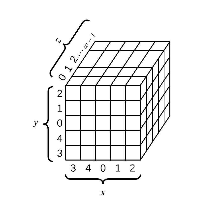
All transformations of the Keccak function are done on the above 3-D array, the numbering of the indices is defined in FIPS 202. This 3 dimensional object is a 5-by-5-by-w array (the w in the equation above).
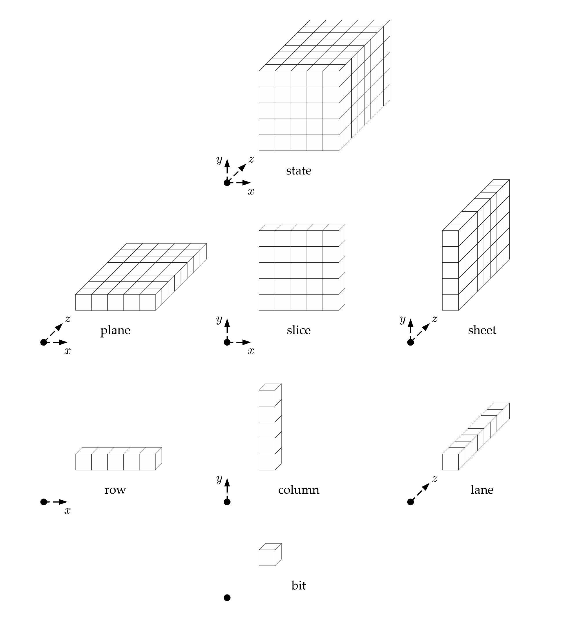
The entire 3-D array is called a state and various other parts of the state array are denoted above.
Capacity and Rate
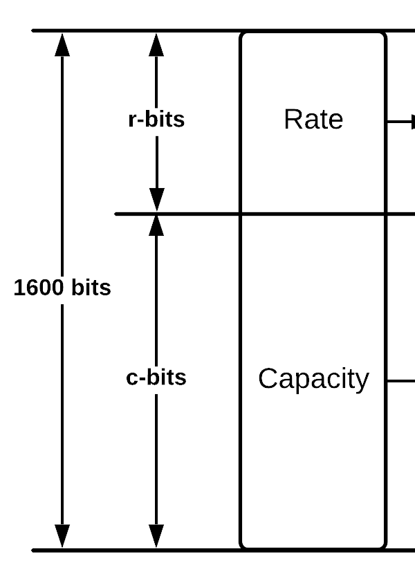
For the main Keccak implantation b is usually restricted to 1600-bits, this gives us a selection of 4 SHA-3 hash functions each with a different output size. This obviously disregards the SHAKE implementations that can have an output of any length.
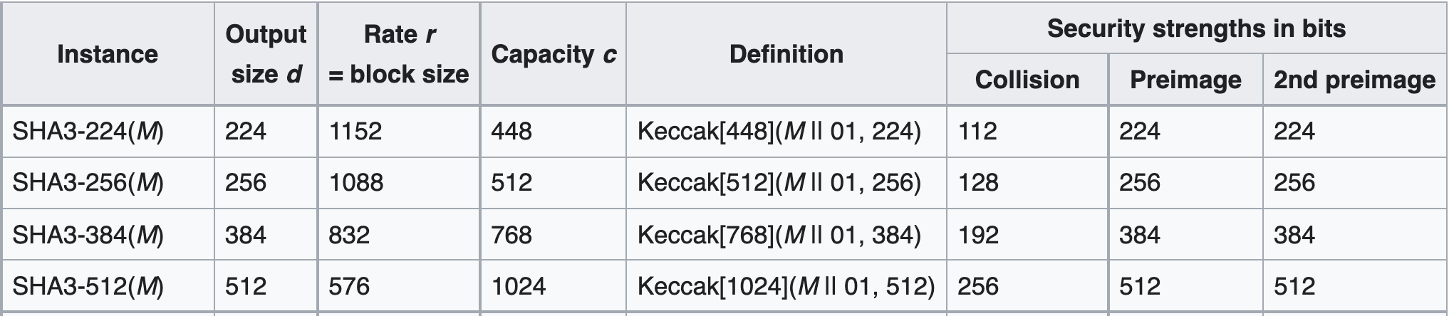
Above is a table of the four NIST standard SHA-3 functions, as you can see for each instance r+c=1600.
Rate – sometimes called bit rate is the size of data blocks that will be absorbed by the function
Capacity – is the area of bits that is untouched by the input or output, meaning new absorption of data will not change these bits. However the function on the newly absorbed data will. None of the capacity bits are used for output of the hash function. The size of the capacity is directly related to how secure the instance is.
The Block Transformation
The block transformation, which is represented as the block labeled function in the above sponge function diagram is broken up in to 5 steps that are done a number of rounds.

The 5 steps are:
- θ (theta)
- ρ (rho)
- π (pi)
- χ (chi)
- ι (iota)
In SHA-3 since we have ℓ = 6, we will do this block transformation 24 rounds for each time the function is run. The round, denoted by ir starts at 0, and is incremented by 1 each time the iota step finishes. Once ir =24, the output of the iota function will be the new capacity and rate This means that if we have twice the amount of bits to hash as the rate bits allow we must run the function 48 times, 24 times for each rate block input, r1 and r2 respectively in the sponge function diagram above.
The θ (theta) Step
The θ step consists of two separate functions, the C function and the D function.
θ C Function
The C function is probably one of the easiest to grasp conceptually. It consists of 4 stages of consecutive XOR calculations.
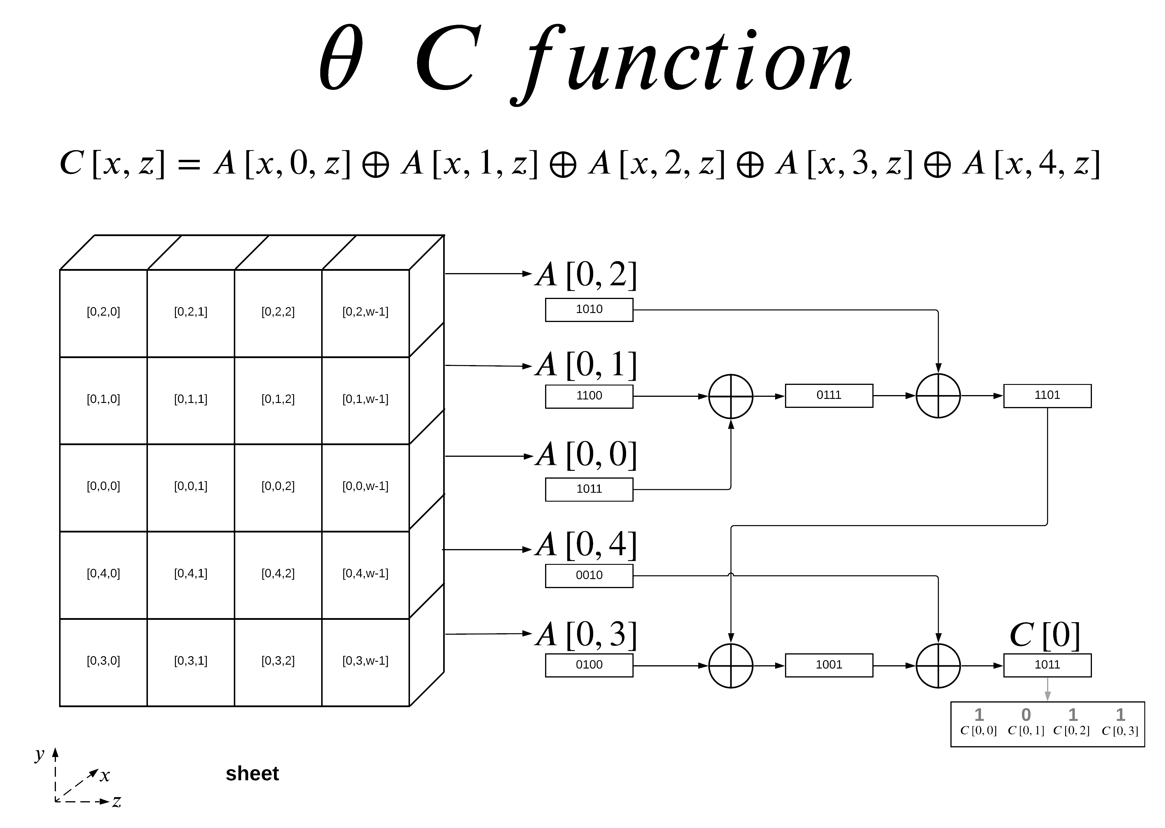
In the example able I show the C function calculation for x=0. We can bulk calculate with respect to the z axis and give the results per lane as shown in the final 4 bit array. The output of the C function for x=0 with with respect to z is broken down below showing the mapping per bit.
θ D Function
The D function introduces cross slice diffusion via the right bitwise rotation with respect to z. It takes two offset C function outputs and XOR’s them together.
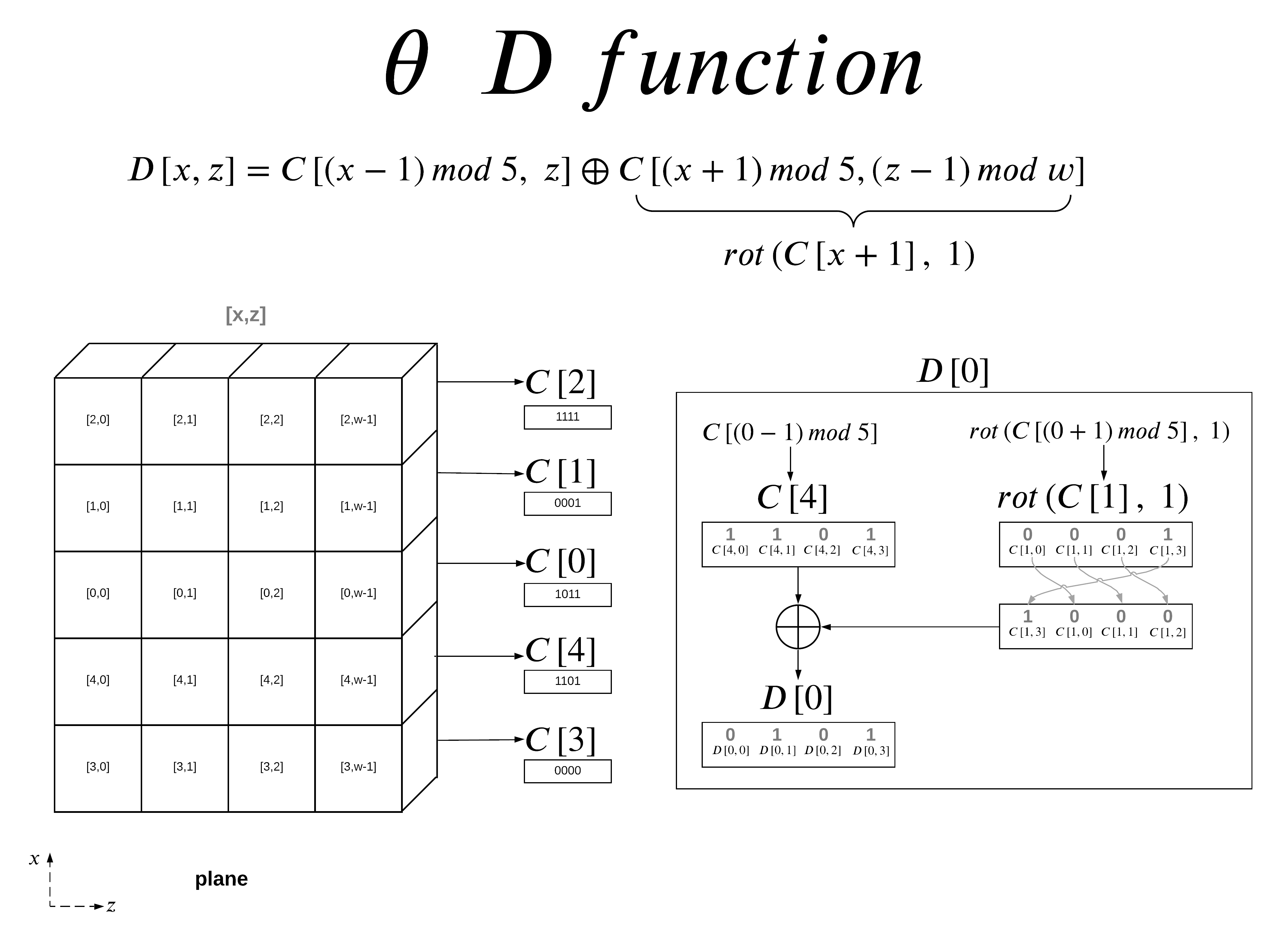
In this example I am showing the D function calculation for x=0. The visual representation of the array has changed axis to show a plane, and the values are the output from the C function. The C value has no y-axis values since it XOR’s each column together, you can think of the C function as the bitwise sum in the y-direction, effectively squishing our state into a single plane.
For D[0], you can see that it does not use C[0], it actually uses the x+1 and x-1 offset of of C[0]. This provides diffusion across the x-direction.
The second argument to the D function offsets z by one position, while you can just do z-1 when calculating an individual bit, when you calculate an entire lane we can represent this z offset as a right-rotation. This provides diffusion across the z-direction.
The final step is to XOR both arguments together, giving you D[0] the lane representation of the D function output for x=0. The mapping per bit is broken down for D[0] to show mapping per bit.
θ Output
The output of the theta function is the XORed result of the initial state array A and the output of the D function.
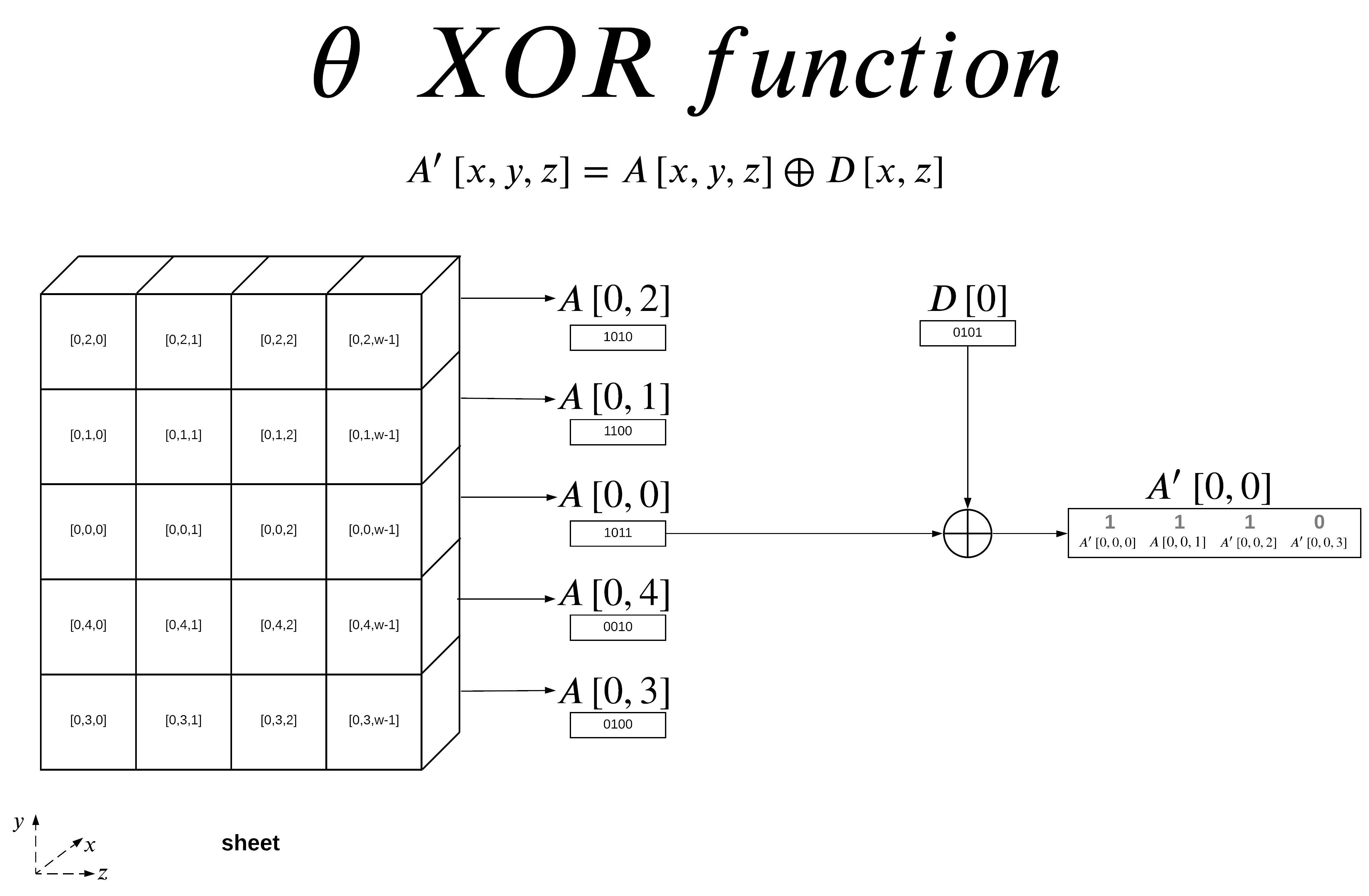
In this example I am showing the final θ XOR output for x=0 and y=0, since D[x,z] does not have a y-component, we end up using D[0] for all subsequent XOR’s when x=0 regardless of y-value.
We can calculate this like our previous examples on a lane (respect to z-axis). The output of the function is labeled A’ (A-prime) which has a size of 5-by-5-by-w bits (the same size as the initial state). A’ is then fed into the ρ (rho) step.
The ρ (rho) Step
The ρ step thankfully only consist of one step. This step is conceptually easy to apply but difficult to understand when written in math notation. We will use A as the input state and A’ as the modified state. In this case A is the output from the final θ step above.
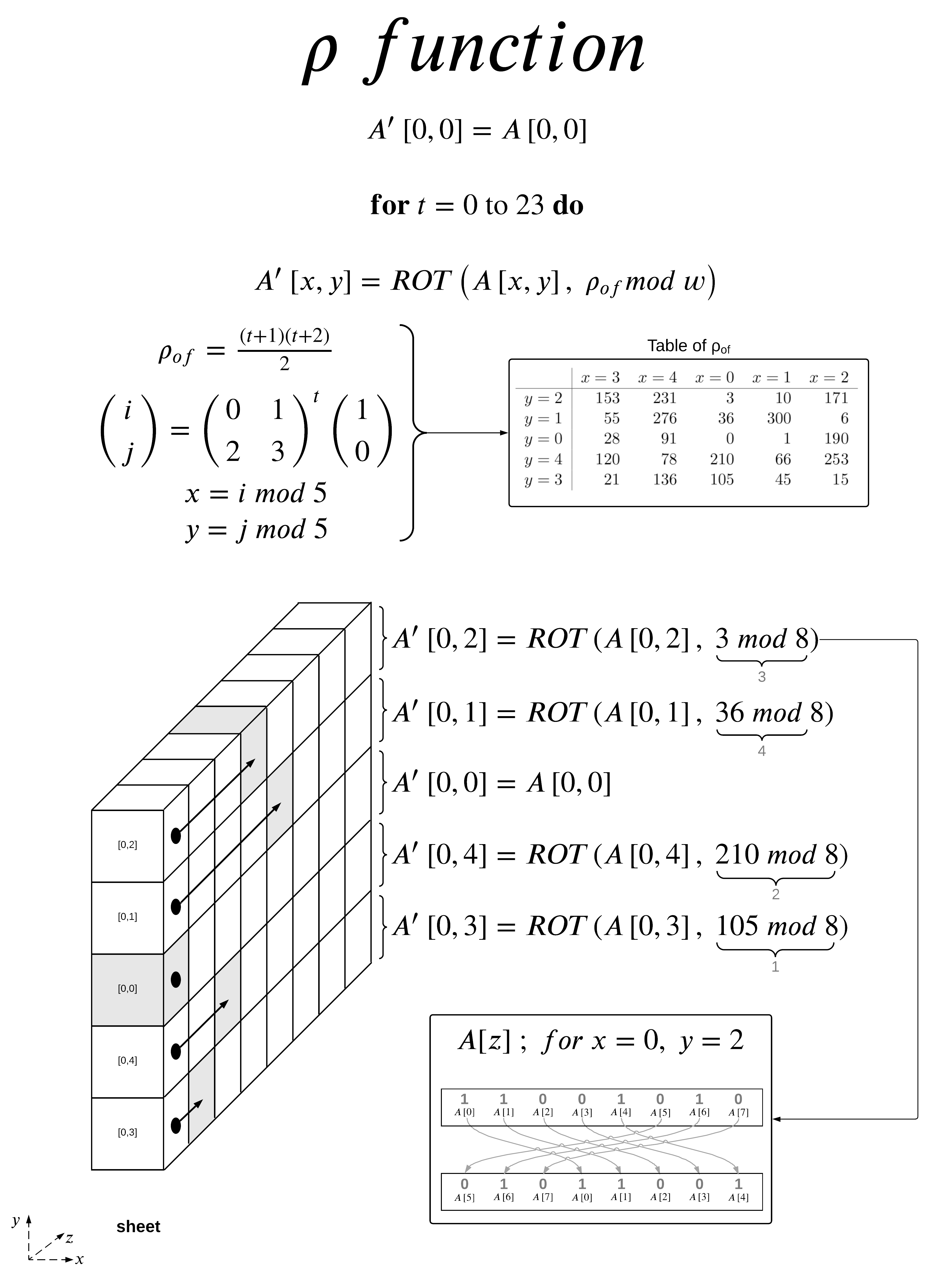
In my example I took the sheet when x=0 and w=8 then applied the ρ function to that sheet. The function is quite simple to apply if you have the table, I also gave the derivation of the table which I will show an example calculation later for a value of t.
Basically for A[0,0] you rotate it 0-bits so it stays the same. To find the rotation for A[0,2] we look at the table and find where x=0 and y=2 intersect, in this case we get 3. We will then rotate the bits in lane A[0,2] by 3-bits to the right, this is visually represented by a dot (its initial position) with an arrow pointing to a grey box (its final position). I also gave a visual representation of the rotation for A[0,2]. This rotation is then preformed on all lanes in the 5-by-5-by-w state.
In order to be able to explain how the ρ offset table is generate we need to understand how matrix multiplication works.
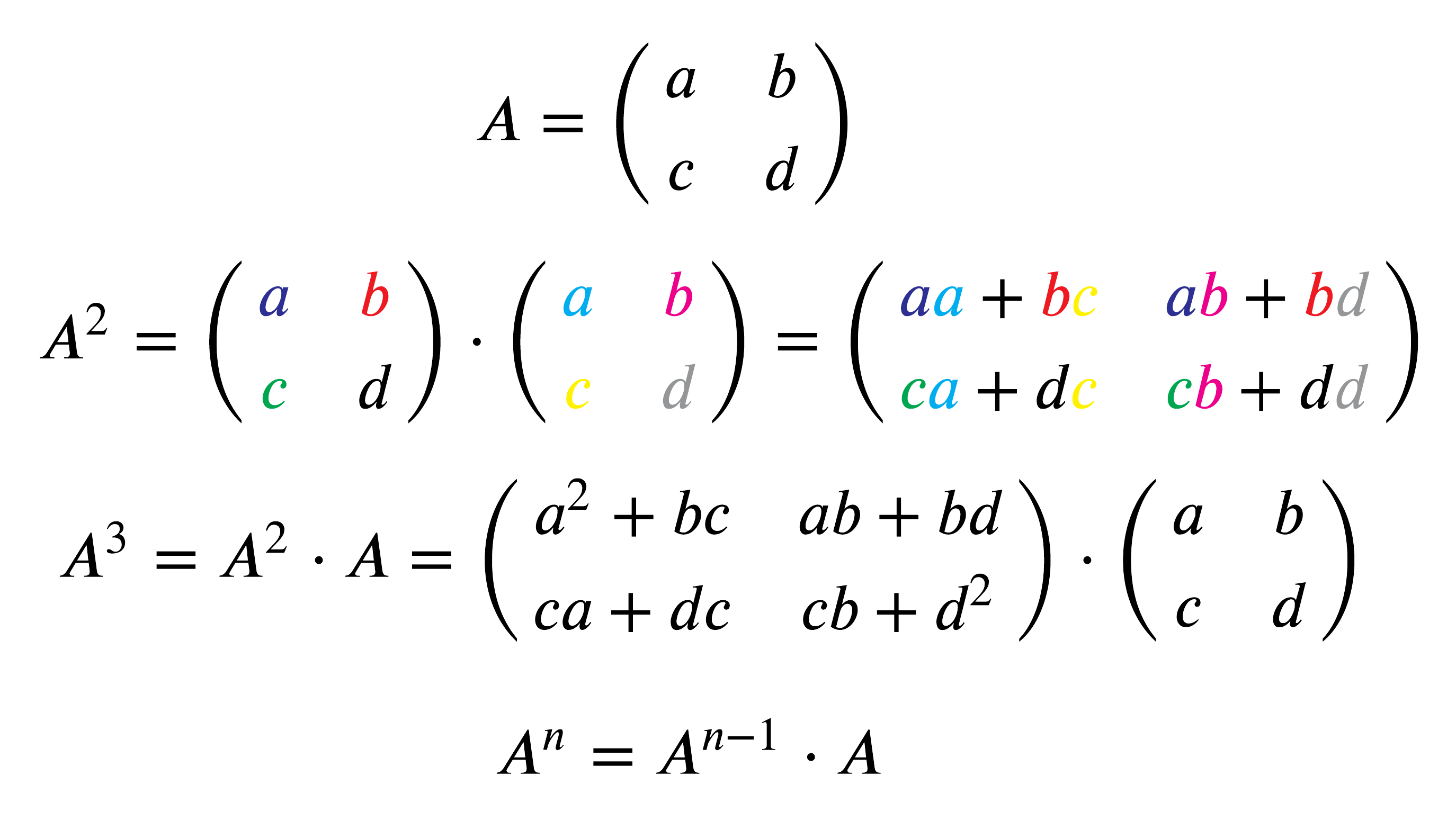
Matrix multiplication is pretty simple, just follow the pretty colors. In order to raise a matrix to the exponent you multiply the n-1 exponential matrix by the initial matrix, since matrix multiplication is not commutative you can’t go the other way.
Now that you have a rough understanding we can do a sample calculation for ρ offset, x and y for when t=10.
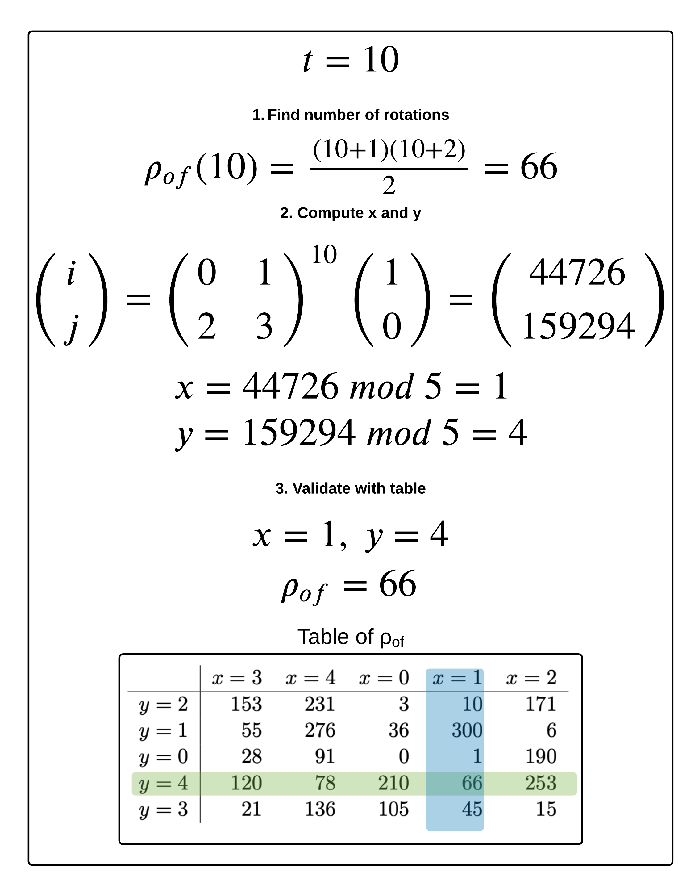
First we plug in 10 into the ρ offset, which gives us a 66-bit rotation. Now we need to know what lane this rotation is referring to. We plugin 10 into our matrix equation and with the help of wolframalpha we get our values for i and j. We then take the mod 5 of each of these values and we end up with x=1 and y=4. We can verify that for these x and y values on the table we have a 66-bit rotation.
With this information you can now just trust the table and forget the matrix algebra you just learned.
The π(pi) step
The π step is actually quite simple as well, the wording of the mathematical function confused me a bit to begin with but, once you get it, it’s pretty straight forward.
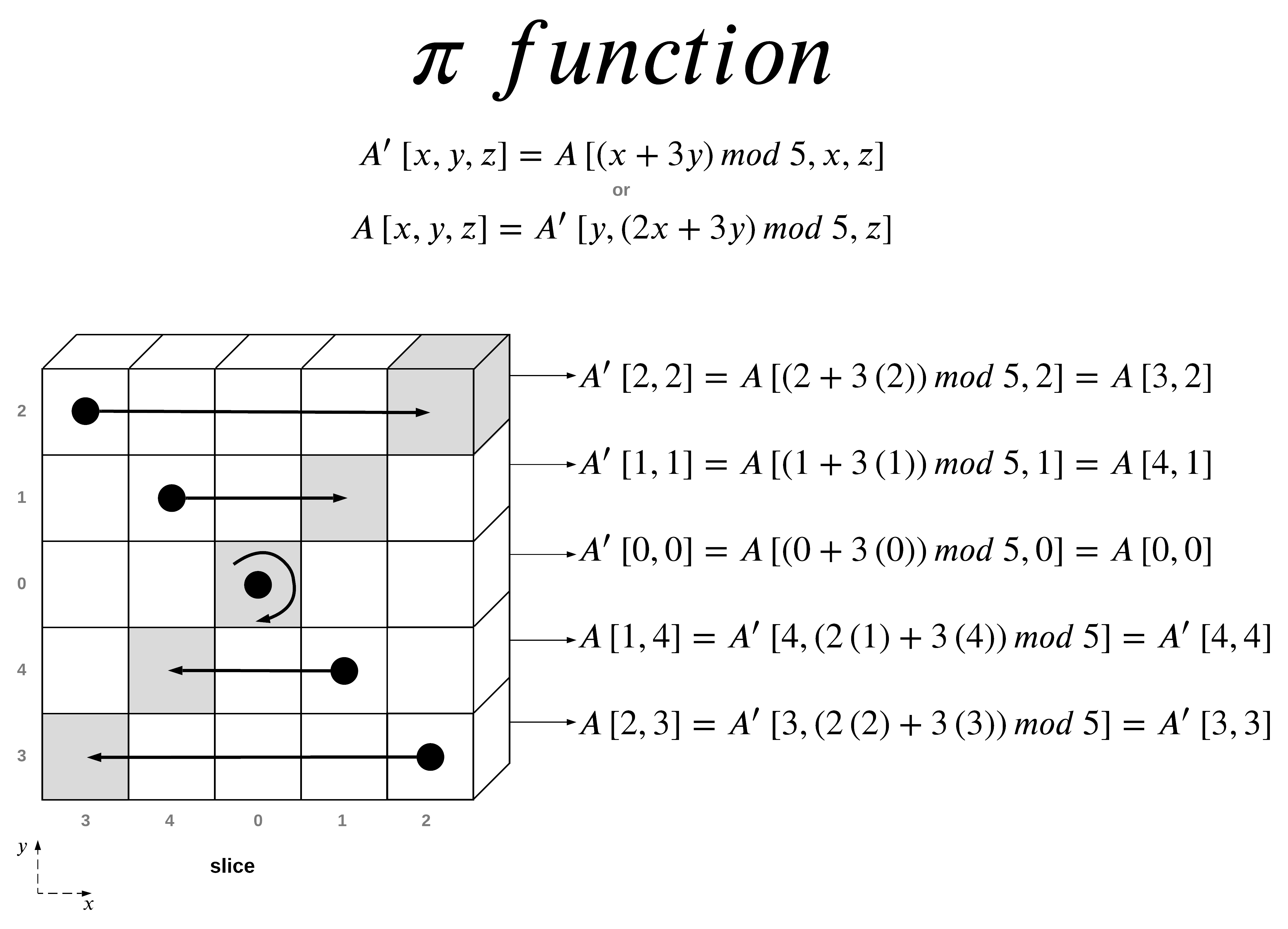
I decided to use the first example of the π function that was given in the NIST FIPS 202 publication of SHA-3. The π function is applied specifically to the diagonal points on a the slice listed above. The function rearranges the positions of lanes in the state.
I decided to list two different versions of the function, the first one, which was take from the official specification and the second one taken from the pseudo-code implementation. While they both do the same thing, the inputs differ.
The first function takes in the location from the output state and gives you the input state location from where it was moved from.
The second function takes in the input state location and gives you where to move it to for the output state.
I have used both functions in the calculations to show that they both do the same thing.

Above are the illustrations taken from the SHA-3 specification that show the π function being applied to all x and y positions.
The χ (chi) Step
The χ step is the only nonlinear mapping step in. It consists for XOR, NOT, and AND operations with bits across the x-direction and is applied to a plane at a time.
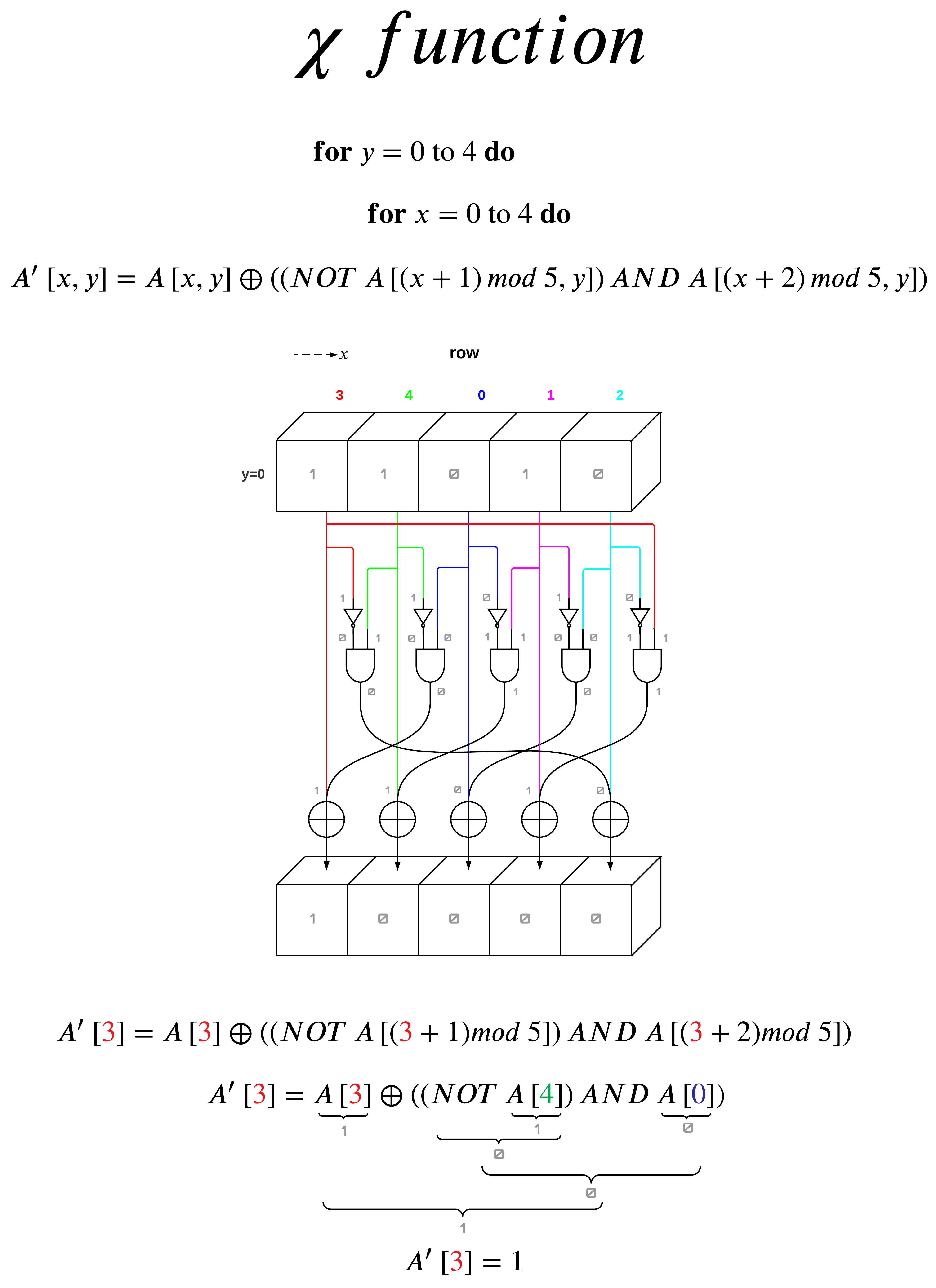
I decided to apply the function to a row instead of a plane to reduce clutter in visualization. I also color coded the x values to help contrast where each logic gate input gets its input value.
The function loop translates to do the χ function on one sheet at a time for all y values.
The ι (iota) Step
The ι step is the most simple of all the steps. The purpose of the ι step is to modify some of the bits of Lane(0,0), the other 24 lanes are not affected by ι. This is done by XORing Lane(0,0) by the round constant (RC[ir]).
Although the ι step is the most simple, it took me the longest to understand, specifically understanding how to generate the round constant vs using the supplied table.
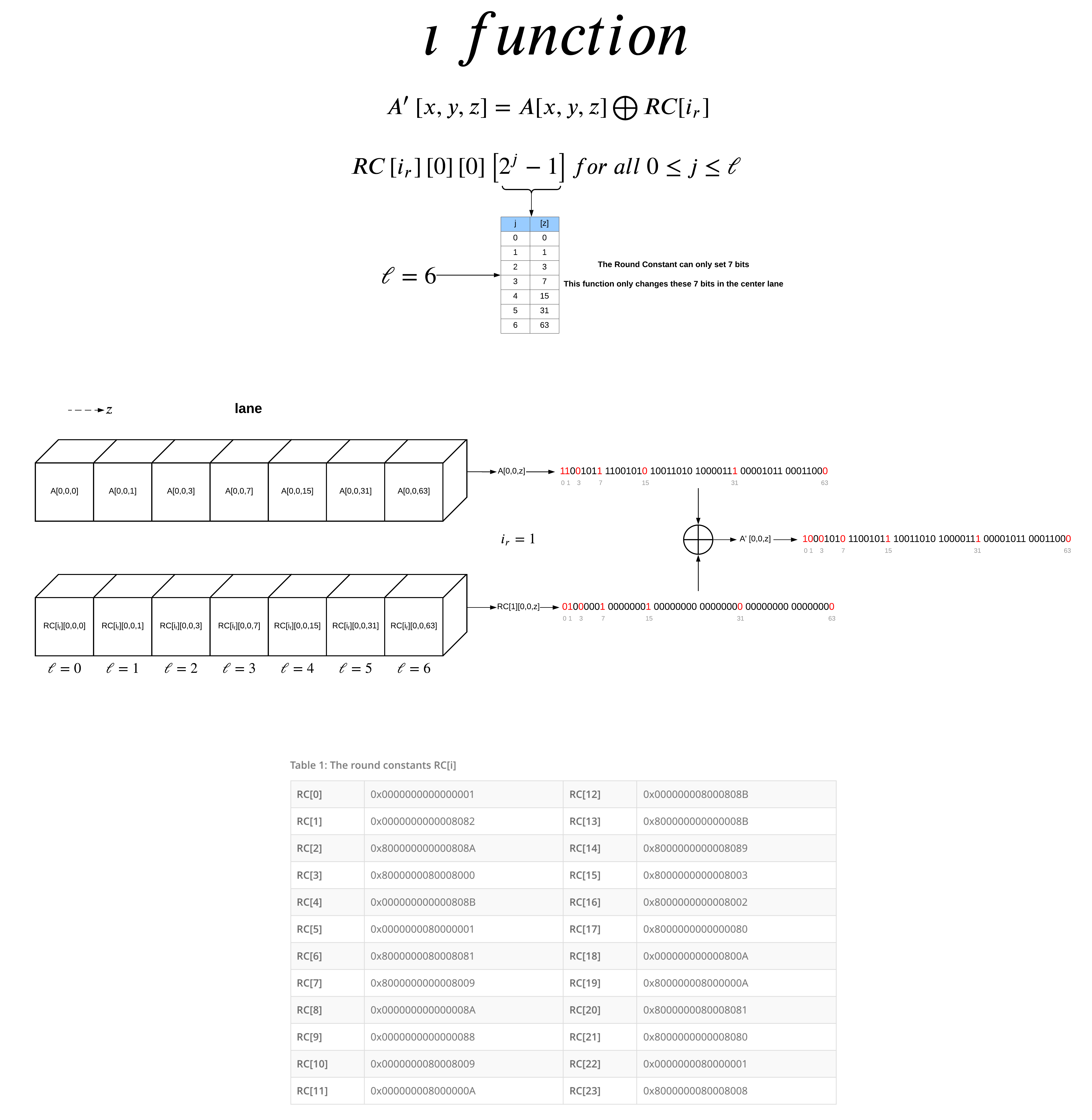
If the case of ℓ=6, the z-position for the RC is given by the first table. The table shows the 7-bits which can be set and their position in the 2ℓ-1 length lane. For the visual representation I show only 7-bits because the rest of the bits are always 0 for the round constant and since they are 0 do not change the initial lane at positions other then the 7-bits.
In this example, ir was chosen to be 1, meaning this is the second round of the block transformation.
The round constants table gives the round constant lane for each value of ir from 0 to 24, represented in hexadecimal format.
I have highlighted the 7-bits can be set for the XOR process to better highlight what is happening.
Coming from a Chemical Engineering background I usually want to understand where constants and equations are derived from before trusting them. Generally because things explode or fail catastrophically when you’re wrong. So, I decided to try to understand how the round constants were calculated.

This took me way longer to understand and required me to learn about linear-feedback shift registers (LFSR). There are a few ways to calculate LFSRs given a the representative polynomial, you can apply it as a Fibonacci or Galois LFSR. I had a lot of trouble since neither of these were referenced in the SHA-3 documentation.
I finally ended up figuring out the round constants were generated using a Galois LFSR with the bit shift direction flipped.
In the above example I gave calculations of RC[0] and RC[1], I think most of the diagram is self explanatory and not much needs to be explained in text. The only thing being that the polynomial degrees represent the bit position of the “taps” of the LFSR.
After the ι step ir is incremented by 1 and the output of the ι step is the new input to the θ step. Once ir is 24 the output of the ι step is the new rate and capacity. This new state is then XORed with any remaining rate chunks and fed into the function again. See the Sponge Construction section for next steps.